25. A First Look at the Kalman Filter #

Contents

A First Look at the Kalman Filter

In addition to what’s in Anaconda, this lecture will need the following libraries:

!pip install quantecon

25.1. Overview #

This lecture provides a simple and intuitive introduction to the Kalman filter, for those who either

have heard of the Kalman filter but don’t know how it works, or
know the Kalman filter equations, but don’t know where they come from

For additional (more advanced) reading on the Kalman filter, see

[Ljungqvist and Sargent, 2018], section 2.7
[Anderson and Moore, 2005]

The second reference presents a comprehensive treatment of the Kalman filter.

Required knowledge: Familiarity with matrix manipulations, multivariate normal distributions, covariance matrices, etc.

We’ll need the following imports:

import matplotlib.pyplot as plt
from scipy import linalg
import numpy as np
import matplotlib.cm as cm
from quantecon import Kalman, LinearStateSpace
from scipy.stats import norm
from scipy.integrate import quad
from scipy.linalg import eigvals

25.2. The Basic Idea #

The Kalman filter has many applications in economics, but for now let’s pretend that we are rocket scientists.

A missile has been launched from country Y and our mission is to track it.

Let $x \in R^{2}$ denote the current location of the missile—a pair indicating latitude-longitude coordinates on a map.

At the present moment in time, the precise location $x$ is unknown, but we do have some beliefs about $x$ .

One way to summarize our knowledge is a point prediction $\hat{x}$

But what if the President wants to know the probability that the missile is currently over the Sea of Japan?
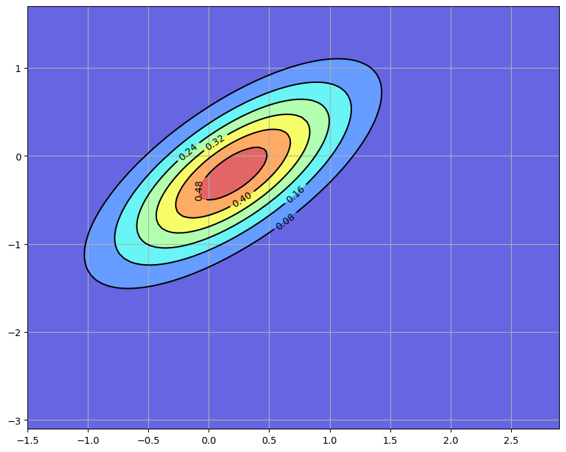
Then it is better to summarize our initial beliefs with a bivariate probability density $p$
- $\int_{E} p (x) d x$ indicates the probability that we attach to the missile being in region $E$ .

The density $p$ is called our prior for the random variable $x$ .

To keep things tractable in our example, we assume that our prior is Gaussian.

In particular, we take

(25.1)#

p = N (\hat{x}, Σ)

where $\hat{x}$ is the mean of the distribution and $Σ$ is a $2 \times 2$ covariance matrix. In our simulations, we will suppose that

(25.2)#

\begin{array}{r} \hat{x} = (\begin{array}{c} 0.2 \\ - 0.2 \end{array}), Σ = (\begin{array}{cc} 0.4 & 0.3 \\ 0.3 & 0.45 \end{array}) \end{array}

This density $p (x)$ is shown below as a contour map, with the center of the red ellipse being equal to $\hat{x}$ .

# Set up the Gaussian prior density p
Σ = [[0.4, 0.3], [0.3, 0.45]]
Σ = np.matrix(Σ)
x_hat = np.matrix([0.2, -0.2]).T
# Define the matrices G and R from the equation y = G x + N(0, R)
G = [[1, 0], [0, 1]]
G = np.matrix(G)
R = 0.5 * Σ
# The matrices A and Q
A = [[1.2, 0], [0, -0.2]]
A = np.matrix(A)
Q = 0.3 * Σ
# The observed value of y
y = np.matrix([2.3, -1.9]).T

# Set up grid for plotting
x_grid = np.linspace(-1.5, 2.9, 100)
y_grid = np.linspace(-3.1, 1.7, 100)
X, Y = np.meshgrid(x_grid, y_grid)

def bivariate_normal(x, y, σ_x=1.0, σ_y=1.0, μ_x=0.0, μ_y=0.0, σ_xy=0.0):
    """
    Compute and return the probability density function of bivariate normal
    distribution of normal random variables x and y

    Parameters
    ----------
    x : array_like(float)
        Random variable

    y : array_like(float)
        Random variable

    σ_x : array_like(float)
          Standard deviation of random variable x

    σ_y : array_like(float)
          Standard deviation of random variable y

    μ_x : scalar(float)
          Mean value of random variable x

    μ_y : scalar(float)
          Mean value of random variable y

    σ_xy : array_like(float)
           Covariance of random variables x and y

    """

    x_μ = x - μ_x
    y_μ = y - μ_y

    ρ = σ_xy / (σ_x * σ_y)
    z = x_μ**2 / σ_x**2 + y_μ**2 / σ_y**2 - 2 * ρ * x_μ * y_μ / (σ_x * σ_y)
    denom = 2 * np.pi * σ_x * σ_y * np.sqrt(1 - ρ**2)
    return np.exp(-z / (2 * (1 - ρ**2))) / denom

def gen_gaussian_plot_vals(μ, C):
    "Z values for plotting the bivariate Gaussian N(μ, C)"
    m_x, m_y = float(μ[0,0]), float(μ[1,0])
    s_x, s_y = np.sqrt(C[0, 0]), np.sqrt(C[1, 1])
    s_xy = C[0, 1]
    return bivariate_normal(X, Y, s_x, s_y, m_x, m_y, s_xy)

# Plot the figure

fig, ax = plt.subplots(figsize=(10, 8))
ax.grid()

Z = gen_gaussian_plot_vals(x_hat, Σ)
ax.contourf(X, Y, Z, 6, alpha=0.6, cmap=cm.jet)
cs = ax.contour(X, Y, Z, 6, colors="black")
ax.clabel(cs, inline=1, fontsize=10)

plt.show()

_images/443146058b8ef11ad00350b41acfa3e0dbd08e4c355c5395aec60813d6316de3.png

25.2.1. The Filtering Step#

We are now presented with some good news and some bad news.

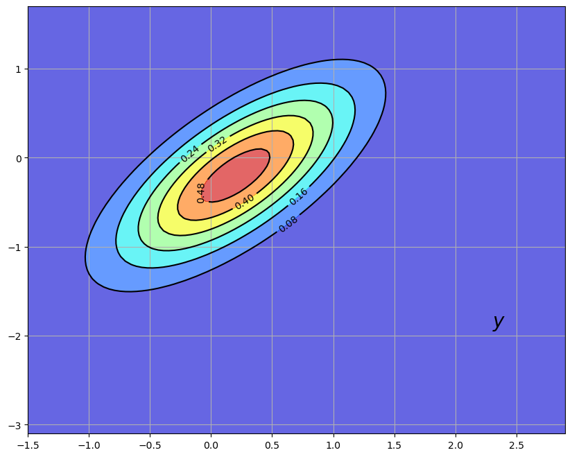
The good news is that the missile has been located by our sensors, which report that the current location is $y = (2.3, - 1.9)$ .

The next figure shows the original prior $p (x)$ and the new reported location $y$

fig, ax = plt.subplots(figsize=(10, 8))
ax.grid()

Z = gen_gaussian_plot_vals(x_hat, Σ)
ax.contourf(X, Y, Z, 6, alpha=0.6, cmap=cm.jet)
cs = ax.contour(X, Y, Z, 6, colors="black")
ax.clabel(cs, inline=1, fontsize=10)
ax.text(float(y[0].item()), float(y[1].item()), "$y$", fontsize=20, color="black")

plt.show()

_images/8d2700dd5eb01924082411edbab3dfe71cf9ee1176020dabe00b48196944ab03.png

The bad news is that our sensors are imprecise.

In particular, we should interpret the output of our sensor not as $y = x$ , but rather as

(25.3)#

y = G x + v, where v \sim N (0, R)

Here $G$ and $R$ are $2 \times 2$ matrices with $R$ positive definite. Both are assumed known, and the noise term $v$ is assumed to be independent of $x$ .

How then should we combine our prior $p (x) = N (\hat{x}, Σ)$ and this new information $y$ to improve our understanding of the location of the missile?

As you may have guessed, the answer is to use Bayes’ theorem, which tells us to update our prior $p (x)$ to $p (x | y)$ via

p (x | y) = \frac{p (y | x) p (x)}{p (y)}

where $p (y) = \int p (y | x) p (x) d x$ .

In solving for $p (x | y)$ , we observe that

$p (x) = N (\hat{x}, Σ)$ .
In view of (25.3), the conditional density $p (y | x)$ is $N (G x, R)$ .
$p (y)$ does not depend on $x$ , and enters into the calculations only as a normalizing constant.

Because we are in a linear and Gaussian framework, the updated density can be computed by calculating population linear regressions.

In particular, the solution is known 1 to be

p (x | y) = N ({\hat{x}}^{F}, Σ^{F})

where

(25.4)#

{\hat{x}}^{F} := \hat{x} + Σ G^{'} (G Σ G^{'} + R)^{- 1} (y - G \hat{x}) and Σ^{F} := Σ - Σ G^{'} (G Σ G^{'} + R)^{- 1} G Σ

Here $Σ G^{'} (G Σ G^{'} + R)^{- 1}$ is the matrix of population regression coefficients of the hidden object $x - \hat{x}$ on the surprise $y - G \hat{x}$ .

This new density $p (x | y) = N ({\hat{x}}^{F}, Σ^{F})$ is shown in the next figure via contour lines and the color map.

The original density is left in as contour lines for comparison

fig, ax = plt.subplots(figsize=(10, 8))
ax.grid()

Z = gen_gaussian_plot_vals(x_hat, Σ)
cs1 = ax.contour(X, Y, Z, 6, colors="black")
ax.clabel(cs1, inline=1, fontsize=10)
M = Σ * G.T * linalg.inv(G * Σ * G.T + R)
x_hat_F = x_hat + M * (y - G * x_hat)
Σ_F = Σ - M * G * Σ
new_Z = gen_gaussian_plot_vals(x_hat_F, Σ_F)
cs2 = ax.contour(X, Y, new_Z, 6, colors="black")
ax.clabel(cs2, inline=1, fontsize=10)
ax.contourf(X, Y, new_Z, 6, alpha=0.6, cmap=cm.jet)
ax.text(float(y[0].item()), float(y[1].item()), "$y$", fontsize=20, color="black")

plt.show()

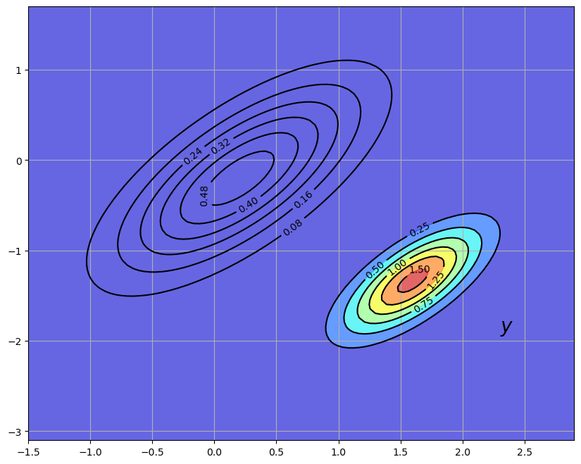
_images/d0f948096a91d708aaca8f22daa835287a8c51afff7f2f848550241121ebc0e6.png

Our new density twists the prior $p (x)$ in a direction determined by the new information $y - G \hat{x}$ .

In generating the figure, we set $G$ to the identity matrix and $R = 0.5 Σ$ for $Σ$ defined in (25.2).

25.2.2. The Forecast Step#

What have we achieved so far?

We have obtained probabilities for the current location of the state (missile) given prior and current information.

This is called “filtering” rather than forecasting because we are filtering out noise rather than looking into the future.

$p (x | y) = N ({\hat{x}}^{F}, Σ^{F})$ is called the filtering distribution

But now let’s suppose that we are given another task: to predict the location of the missile after one unit of time (whatever that may be) has elapsed.

To do this we need a model of how the state evolves.

Let’s suppose that we have one, and that it’s linear and Gaussian. In particular,

(25.5)#

x_{t + 1} = A x_{t} + w_{t + 1}, where w_{t} \sim N (0, Q)

Our aim is to combine this law of motion and our current distribution $p (x | y) = N ({\hat{x}}^{F}, Σ^{F})$ to come up with a new predictive distribution for the location in one unit of time.

In view of (25.5), all we have to do is introduce a random vector $x^{F} \sim N ({\hat{x}}^{F}, Σ^{F})$ and work out the distribution of $A x^{F} + w$ where $w$ is independent of $x^{F}$ and has distribution $N (0, Q)$ .

Since linear combinations of Gaussians are Gaussian, $A x^{F} + w$ is Gaussian.

Elementary calculations and the expressions in (25.4) tell us that

E [A x^{F} + w] = A E x^{F} + E w = A {\hat{x}}^{F} = A \hat{x} + A Σ G^{'} (G Σ G^{'} + R)^{- 1} (y - G \hat{x})

and

Var [A x^{F} + w] = A Var [x^{F}] A^{'} + Q = A Σ^{F} A^{'} + Q = A Σ A^{'} - A Σ G^{'} (G Σ G^{'} + R)^{- 1} G Σ A^{'} + Q

The matrix $A Σ G^{'} (G Σ G^{'} + R)^{- 1}$ is often written as $K_{Σ}$ and called the Kalman gain.

The subscript $Σ$ has been added to remind us that $K_{Σ}$ depends on $Σ$ , but not $y$ or $\hat{x}$ .

Using this notation, we can summarize our results as follows.

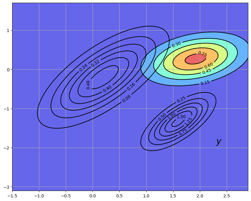
Our updated prediction is the density $N ({\hat{x}}_{n e w}, Σ_{n e w})$ where

(25.6)#

\begin{array}{r} \begin{aligned} {\hat{x}}_{n e w} & := A \hat{x} + K_{Σ} (y - G \hat{x}) \\ Σ_{n e w} & := A Σ A^{'} - K_{Σ} G Σ A^{'} + Q \end{aligned} \end{array}

The density $p_{n e w} (x) = N ({\hat{x}}_{n e w}, Σ_{n e w})$ is called the predictive distribution

The predictive distribution is the new density shown in the following figure, where the update has used parameters.

\begin{array}{r} A = (\begin{array}{cc} 1.2 & 0.0 \\ 0.0 & - 0.2 \end{array}), Q = 0.3 * Σ \end{array}

fig, ax = plt.subplots(figsize=(10, 8))
ax.grid()

# Density 1
Z = gen_gaussian_plot_vals(x_hat, Σ)
cs1 = ax.contour(X, Y, Z, 6, colors="black")
ax.clabel(cs1, inline=1, fontsize=10)

# Density 2
M = Σ * G.T * linalg.inv(G * Σ * G.T + R)
x_hat_F = x_hat + M * (y - G * x_hat)
Σ_F = Σ - M * G * Σ
Z_F = gen_gaussian_plot_vals(x_hat_F, Σ_F)
cs2 = ax.contour(X, Y, Z_F, 6, colors="black")
ax.clabel(cs2, inline=1, fontsize=10)

# Density 3
new_x_hat = A * x_hat_F
new_Σ = A * Σ_F * A.T + Q
new_Z = gen_gaussian_plot_vals(new_x_hat, new_Σ)
cs3 = ax.contour(X, Y, new_Z, 6, colors="black")
ax.clabel(cs3, inline=1, fontsize=10)
ax.contourf(X, Y, new_Z, 6, alpha=0.6, cmap=cm.jet)
ax.text(float(y[0].item()), float(y[1].item()), "$y$", fontsize=20, color="black")

plt.show()

_images/89f2b932ee7101362e260d3d123877f5b030b8cd2ec03040ab78cb09a7e3f83b.png

25.2.3. The Recursive Procedure#

Let’s look back at what we’ve done.

We started the current period with a prior $p (x)$ for the location $x$ of the missile.

We then used the current measurement $y$ to update to $p (x | y)$ .

Finally, we used the law of motion (25.5) for ${x_{t}}$ to update to $p_{n e w} (x)$ .

If we now step into the next period, we are ready to go round again, taking $p_{n e w} (x)$ as the current prior.

Swapping notation $p_{t} (x)$ for $p (x)$ and $p_{t + 1} (x)$ for $p_{n e w} (x)$ , the full recursive procedure is:

Start the current period with prior $p_{t} (x) = N ({\hat{x}}_{t}, Σ_{t})$ .
Observe current measurement $y_{t}$ .
Compute the filtering distribution $p_{t} (x | y) = N ({\hat{x}}_{t}^{F}, Σ_{t}^{F})$ from $p_{t} (x)$ and $y_{t}$ , applying Bayes rule and the conditional distribution (25.3).
Compute the predictive distribution $p_{t + 1} (x) = N ({\hat{x}}_{t + 1}, Σ_{t + 1})$ from the filtering distribution and (25.5).
Increment $t$ by one and go to step 1.

Repeating (25.6), the dynamics for ${\hat{x}}_{t}$ and $Σ_{t}$ are as follows

(25.7)#

\begin{array}{r} \begin{aligned} {\hat{x}}_{t + 1} & = A {\hat{x}}_{t} + K_{Σ_{t}} (y_{t} - G {\hat{x}}_{t}) \\ Σ_{t + 1} & = A Σ_{t} A^{'} - K_{Σ_{t}} G Σ_{t} A^{'} + Q \end{aligned} \end{array}

These are the standard dynamic equations for the Kalman filter (see, for example, [Ljungqvist and Sargent, 2018], page 58).

25.3. Convergence #

The matrix $Σ_{t}$ is a measure of the uncertainty of our prediction ${\hat{x}}_{t}$ of $x_{t}$ .

Apart from special cases, this uncertainty will never be fully resolved, regardless of how much time elapses.

One reason is that our prediction ${\hat{x}}_{t}$ is made based on information available at $t - 1$ , not $t$ .

Even if we know the precise value of $x_{t - 1}$ (which we don’t), the transition equation (25.5) implies that $x_{t} = A x_{t - 1} + w_{t}$ .

Since the shock $w_{t}$ is not observable at $t - 1$ , any time $t - 1$ prediction of $x_{t}$ will incur some error (unless $w_{t}$ is degenerate).

However, it is certainly possible that $Σ_{t}$ converges to a constant matrix as $t \to \infty$ .

To study this topic, let’s expand the second equation in (25.7):

(25.8)#

Σ_{t + 1} = A Σ_{t} A^{'} - A Σ_{t} G^{'} (G Σ_{t} G^{'} + R)^{- 1} G Σ_{t} A^{'} + Q

This is a nonlinear difference equation in $Σ_{t}$ .

A fixed point of (25.8) is a constant matrix $Σ$ such that

(25.9)#

Σ = A Σ A^{'} - A Σ G^{'} (G Σ G^{'} + R)^{- 1} G Σ A^{'} + Q

Equation (25.8) is known as a discrete-time Riccati difference equation.

Equation (25.9) is known as a discrete-time algebraic Riccati equation.

Conditions under which a fixed point exists and the sequence ${Σ_{t}}$ converges to it are discussed in [Anderson et al., 1996] and [Anderson and Moore, 2005], chapter 4.

A sufficient (but not necessary) condition is that all the eigenvalues $λ_{i}$ of $A$ satisfy $| λ_{i} | < 1$ (cf. e.g., [Anderson and Moore, 2005], p. 77).

(This strong condition assures that the unconditional distribution of $x_{t}$ converges as $t \to + \infty$ .)

In this case, for any initial choice of $Σ_{0}$ that is both non-negative and symmetric, the sequence ${Σ_{t}}$ in (25.8) converges to a non-negative symmetric matrix $Σ$ that solves (25.9).

25.4. Implementation #

The class Kalman from the QuantEcon.py package implements the Kalman filter

Instance data consists of:
- the moments $({\hat{x}}_{t}, Σ_{t})$ of the current prior.
- An instance of the LinearStateSpace class from QuantEcon.py.

The latter represents a linear state space model of the form

\begin{array}{r} \begin{aligned} x_{t + 1} & = A x_{t} + C w_{t + 1} \\ y_{t} & = G x_{t} + H v_{t} \end{aligned} \end{array}

where the shocks $w_{t}$ and $v_{t}$ are IID standard normals.

To connect this with the notation of this lecture we set

Q := C C^{'} and R := H H^{'}

The class Kalman from the QuantEcon.py package has a number of methods, some that we will wait to use until we study more advanced applications in subsequent lectures.
Methods pertinent for this lecture are:
- prior_to_filtered, which updates $({\hat{x}}_{t}, Σ_{t})$ to $({\hat{x}}_{t}^{F}, Σ_{t}^{F})$
- filtered_to_forecast, which updates the filtering distribution to the predictive distribution – which becomes the new prior $({\hat{x}}_{t + 1}, Σ_{t + 1})$
- update, which combines the last two methods
- a stationary_values, which computes the solution to (25.9) and the corresponding (stationary) Kalman gain

You can view the program on GitHub.

25.5. Exercises #

Exercise 25.1

Consider the following simple application of the Kalman filter, loosely based on [Ljungqvist and Sargent, 2018], section 2.9.2.

Suppose that

all variables are scalars
the hidden state ${x_{t}}$ is in fact constant, equal to some $θ \in R$ unknown to the modeler

State dynamics are therefore given by (25.5) with $A = 1$ , $Q = 0$ and $x_{0} = θ$ .

The measurement equation is $y_{t} = θ + v_{t}$ where $v_{t}$ is $N (0, 1)$ and IID.

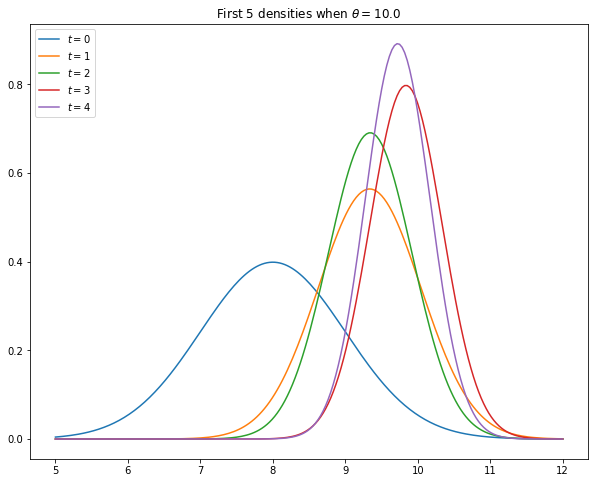
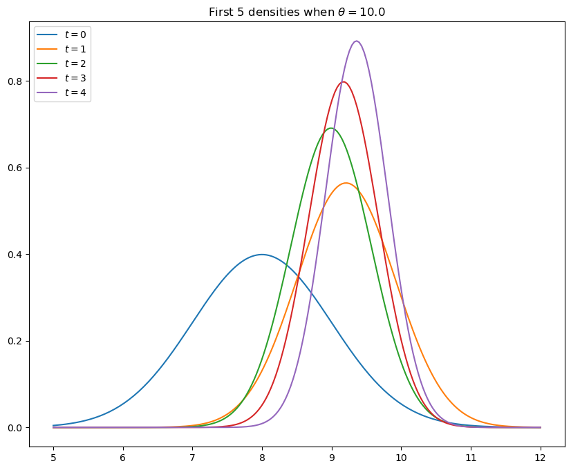
The task of this exercise to simulate the model and, using the code from kalman.py, plot the first five predictive densities $p_{t} (x) = N ({\hat{x}}_{t}, Σ_{t})$ .

As shown in [Ljungqvist and Sargent, 2018], sections 2.9.1–2.9.2, these distributions asymptotically put all mass on the unknown value $θ$ .

In the simulation, take $θ = 10$ , ${\hat{x}}_{0} = 8$ and $Σ_{0} = 1$ .

Your figure should – modulo randomness – look something like this

Solution to Exercise 25.1

# Parameters
θ = 10  # Constant value of state x_t
A, C, G, H = 1, 0, 1, 1
ss = LinearStateSpace(A, C, G, H, mu_0=θ)

# Set prior, initialize kalman filter
x_hat_0, Σ_0 = 8, 1
kalman = Kalman(ss, x_hat_0, Σ_0)

# Draw observations of y from state space model
N = 5
x, y = ss.simulate(N)
y = y.flatten()

# Set up plot
fig, ax = plt.subplots(figsize=(10,8))
xgrid = np.linspace(θ - 5, θ + 2, 200)

for i in range(N):
    # Record the current predicted mean and variance
    m, v = [float(z) for z in (kalman.x_hat.item(), kalman.Sigma.item())]
    # Plot, update filter
    ax.plot(xgrid, norm.pdf(xgrid, loc=m, scale=np.sqrt(v)), label=f'$t={i}$')
    kalman.update(y[i])

ax.set_title(f'First {N} densities when $\\theta = {θ:.1f}$')
ax.legend(loc='upper left')
plt.show()

_images/a8111b3f765e58218ea0988897565e706dad2b65811220331aa0c56ad72827af.png

Exercise 25.2

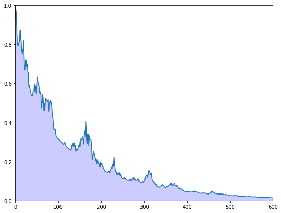
The preceding figure gives some support to the idea that probability mass converges to $θ$ .

To get a better idea, choose a small $ϵ > 0$ and calculate

z_{t} := 1 - \int_{θ - ϵ}^{θ + ϵ} p_{t} (x) d x

for $t = 0, 1, 2, \dots, T$ .

Plot $z_{t}$ against $T$ , setting $ϵ = 0.1$ and $T = 600$ .

Your figure should show error erratically declining something like this

Solution to Exercise 25.2

ϵ = 0.1
θ = 10  # Constant value of state x_t
A, C, G, H = 1, 0, 1, 1
ss = LinearStateSpace(A, C, G, H, mu_0=θ)

x_hat_0, Σ_0 = 8, 1
kalman = Kalman(ss, x_hat_0, Σ_0)

T = 600
z = np.empty(T)
x, y = ss.simulate(T)
y = y.flatten()

for t in range(T):
    # Record the current predicted mean and variance and plot their densities
    m, v = [float(temp) for temp in (kalman.x_hat.item(), kalman.Sigma.item())]

    f = lambda x: norm.pdf(x, loc=m, scale=np.sqrt(v))
    integral, error = quad(f, θ - ϵ, θ + ϵ)
    z[t] = 1 - integral

    kalman.update(y[t])

fig, ax = plt.subplots(figsize=(9, 7))
ax.set_ylim(0, 1)
ax.set_xlim(0, T)
ax.plot(range(T), z)
ax.fill_between(range(T), np.zeros(T), z, color="blue", alpha=0.2)
plt.show()

_images/fca075b64d98755d8c22cacea10fd163a633f365ac48c10af7da53ecb62b728b.png

Exercise 25.3

As discussed above, if the shock sequence ${w_{t}}$ is not degenerate, then it is not in general possible to predict $x_{t}$ without error at time $t - 1$ (and this would be the case even if we could observe $x_{t - 1}$ ).

Let’s now compare the prediction ${\hat{x}}_{t}$ made by the Kalman filter against a competitor who is allowed to observe $x_{t - 1}$ .

This competitor will use the conditional expectation $E [x_{t} | x_{t - 1}]$ , which in this case is $A x_{t - 1}$ .

The conditional expectation is known to be the optimal prediction method in terms of minimizing mean squared error.

(More precisely, the minimizer of $E ‖ x_{t} - g (x_{t - 1}) ‖^{2}$ with respect to $g$ is $g^{*} (x_{t - 1}) := E [x_{t} | x_{t - 1}]$ )

Thus we are comparing the Kalman filter against a competitor who has more information (in the sense of being able to observe the latent state) and behaves optimally in terms of minimizing squared error.

Our horse race will be assessed in terms of squared error.

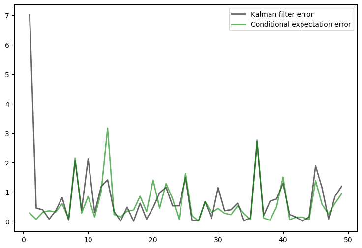
In particular, your task is to generate a graph plotting observations of both $‖ x_{t} - A x_{t - 1} ‖^{2}$ and $‖ x_{t} - {\hat{x}}_{t} ‖^{2}$ against $t$ for $t = 1, \dots, 50$ .

For the parameters, set $G = I, R = 0.5 I$ and $Q = 0.3 I$ , where $I$ is the $2 \times 2$ identity.

Set

\begin{array}{r} A = (\begin{array}{cc} 0.5 & 0.4 \\ 0.6 & 0.3 \end{array}) \end{array}

To initialize the prior density, set

\begin{array}{r} Σ_{0} = (\begin{array}{cc} 0.9 & 0.3 \\ 0.3 & 0.9 \end{array}) \end{array}

and ${\hat{x}}_{0} = (8, 8)$ .

Finally, set $x_{0} = (0, 0)$ .

You should end up with a figure similar to the following (modulo randomness)

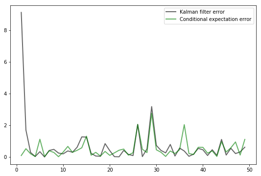
Observe how, after an initial learning period, the Kalman filter performs quite well, even relative to the competitor who predicts optimally with knowledge of the latent state.

Solution to Exercise 25.3

# Define A, C, G, H
G = np.identity(2)
H = np.sqrt(0.5) * np.identity(2)

A = [[0.5, 0.4],
     [0.6, 0.3]]
C = np.sqrt(0.3) * np.identity(2)

# Set up state space mode, initial value x_0 set to zero
ss = LinearStateSpace(A, C, G, H, mu_0 = np.zeros(2))

# Define the prior density
Σ = [[0.9, 0.3],
     [0.3, 0.9]]
Σ = np.array(Σ)
x_hat = np.array([8, 8])

# Initialize the Kalman filter
kn = Kalman(ss, x_hat, Σ)

# Print eigenvalues of A
print("Eigenvalues of A:")
print(eigvals(A))

# Print stationary Σ
S, K = kn.stationary_values()
print("Stationary prediction error variance:")
print(S)

# Generate the plot
T = 50
x, y = ss.simulate(T)

e1 = np.empty(T-1)
e2 = np.empty(T-1)

for t in range(1, T):
    kn.update(y[:,t])
    e1[t-1] = np.sum((x[:, t] - kn.x_hat.flatten())**2)
    e2[t-1] = np.sum((x[:, t] - A @ x[:, t-1])**2)

fig, ax = plt.subplots(figsize=(9,6))
ax.plot(range(1, T), e1, 'k-', lw=2, alpha=0.6,
        label='Kalman filter error')
ax.plot(range(1, T), e2, 'g-', lw=2, alpha=0.6,
        label='Conditional expectation error')
ax.legend()
plt.show()

Eigenvalues of A:
[ 0.9+0.j -0.1+0.j]
Stationary prediction error variance:
[[0.40329108 0.1050718 ]
 [0.1050718  0.41061709]]

_images/799416fcf4a31b0aec5b2fc0d8929f2a076425819b71bfe24d5009d0f10fa407.png

Exercise 25.4

Try varying the coefficient $0.3$ in $Q = 0.3 I$ up and down.

Observe how the diagonal values in the stationary solution $Σ$ (see (25.9)) increase and decrease in line with this coefficient.

The interpretation is that more randomness in the law of motion for $x_{t}$ causes more (permanent) uncertainty in prediction.

1: See, for example, page 93 of [Bishop, 2006]. To get from his expressions to the ones used above, you will also need to apply the Woodbury matrix identity.

25. A First Look at the Kalman Filter#

25.1. Overview#

25.2. The Basic Idea#

25.2.1. The Filtering Step#

25.2.2. The Forecast Step#

25.2.3. The Recursive Procedure#

25.3. Convergence#

25.4. Implementation#

25.5. Exercises#