60. The Permanent Income Model#

60.2.1. Preliminaries#

We use a class of stochastic processes called martingales.

A discrete-time martingale is a stochastic process (i.e., a sequence of random variables) $\{X_t\}$ with finite mean at each $t$ and satisfying

Here ${\mathbb{E}}_t:=\mathbb{E}[\cdot |{\mathcal{F}}_t]$ is a conditional mathematical expectation conditional on the time $t$ information set ${\mathcal{F}}_t$.

The latter is just a collection of random variables that the modeler declares to be visible at $t$.

• When not explicitly defined, it is usually understood that ${\mathcal{F}}_t=\{X_t,X_{t-1},\dots ,X_0\}$.

Martingales have the feature that the history of past outcomes provides no predictive power for changes between current and future outcomes.

For example, the current wealth of a gambler engaged in a “fair game” has this property.

One common class of martingales is the family of random walks.

A random walk is a stochastic process $\{X_t\}$ that satisfies

for some IID zero mean innovation sequence $\{w_t\}$.

Evidently, $X_t$ can also be expressed as

Not every martingale arises as a random walk (see, for example, Wald’s martingale).

60.2.2. The Decision Problem#

A consumer has preferences over consumption streams that are ordered by the utility functional

where

• ${\mathbb{E}}_t$ is the mathematical expectation conditioned on the consumer’s time $t$ information

• $c_t$ is time $t$ consumption

• $u$ is a strictly concave one-period utility function

• $\beta \in (0,1)$ is a discount factor

The consumer maximizes (60.1) by choosing a consumption, borrowing plan $\{c_t,b_{t+1}{\}}_{t=0}^{\mathrm{\infty }}$ subject to the sequence of budget constraints

Here

• $y_t$ is an exogenous endowment process.

• $r>0$ is a time-invariant risk-free net interest rate.

• $b_t$ is one-period risk-free debt maturing at $t$.

The consumer also faces initial conditions $b_0$ and $y_0$, which can be fixed or random.

60.2.3. Assumptions#

For the remainder of this lecture, we follow Friedman and Hall in assuming that $(1+r{)}^{-1}=\beta$.

Regarding the endowment process, we assume it has the state-space representation

where

• $\{w_t\}$ is an IID vector process with $\mathbb{E}{w}_t=0$ and $\mathbb{E}{w}_t{w}_t^{\prime }=I$.

• The spectral radius of $A$ satisfies $\rho (A)<\sqrt{1/\beta }$.

• $U$ is a selection vector that pins down $y_t$ as a particular linear combination of components of $z_t$.

The restriction on $\rho (A)$ prevents income from growing so fast that discounted geometric sums of some quadratic forms to be described below become infinite.

Regarding preferences, we assume the quadratic utility function

where $\gamma$ is a bliss level of consumption.

Finally, we impose the no Ponzi scheme condition

This condition rules out an always-borrow scheme that would allow the consumer to enjoy bliss consumption forever.

60.2.4. First-Order Conditions#

First-order conditions for maximizing (60.1) subject to (60.2) are

These optimality conditions are also known as Euler equations.

If you’re not sure where they come from, you can find a proof sketch in the appendix.

With our quadratic preference specification, (60.5) has the striking implication that consumption follows a martingale:

(In fact, quadratic preferences are necessary for this conclusion 1.)

One way to interpret (60.6) is that consumption will change only when “new information” about permanent income is revealed.

These ideas will be clarified below.

60.2.5. The Optimal Decision Rule#

Now let’s deduce the optimal decision rule 2.

In doing so, we need to combine

1. the optimality condition (60.6)

2. the period-by-period budget constraint (60.2), and

3. the boundary condition (60.4)

To accomplish this, observe first that (60.4) implies $\underset{t\to \mathrm{\infty }}{lim}{\beta }^{\frac{t}{2}}{b}_{t+1}=0$.

Using this restriction on the debt path and solving (60.2) forward yields

Take conditional expectations on both sides of (60.7) and use the martingale property of consumption and the law of iterated expectations to deduce

Expressed in terms of $c_t$ we get

where the last equality uses $(1+r)\beta =1$.

These last two equations assert that consumption equals economic income

• financial wealth equals $-b_t$

• non-financial wealth equals $\sum _{j=0}^{\mathrm{\infty }}{\beta }^j{\mathbb{E}}_t[y_{t+j}]$

• total wealth equals the sum of financial and non-financial wealth

• a marginal propensity to consume out of total wealth equals the interest factor $\frac{r}{1+r}$

• economic income equals

  • a constant marginal propensity to consume times the sum of non-financial wealth and financial wealth

  • the amount the consumer can consume while leaving its wealth intact

60.2.5.3. A Simple Example with IID Income#

To gain some preliminary intuition on the implications of (60.11), let’s look at a highly stylized example where income is just IID.

(Later examples will investigate more realistic income streams.)

In particular, let $\{w_t{\}}_{t=1}^{\mathrm{\infty }}$ be IID and scalar standard normal, and let

$$\begin{array}{r}{z}_t=\left[\begin{array}{c}{z}_t^1\\ 1\end{array}\right],A=\left[\begin{array}{cc}0& 0\\ 0& 1\end{array}\right],U=\left[\begin{array}{cc}1& \mu \end{array}\right],C=\left[\begin{array}{c}\sigma \\ 0\end{array}\right]\end{array}$$

Finally, let $b_0=z_0^1=0$.

Under these assumptions, we have $y_t=\mu +\sigma w_t\sim N(\mu ,{\sigma }^2)$.

Further, if you work through the state space representation, you will see that

$$\begin{array}{r}\begin{array}{rl}{b}_t& =-\sigma \sum _{j=1}^{t-1}{w}_j\\ c_t& =\mu +(1-\beta )\sigma \sum _{j=1}^t{w}_j\end{array}\end{array}$$

Thus, income is IID and debt and consumption are both Gaussian random walks.

Defining assets as $-b_t$, we see that assets are just the cumulative sum of unanticipated incomes prior to the present date.

The next figure shows a typical realization with $r=0.05$, $\mu =1$, and $\sigma =0.15$

r = 0.05
β = 1 / (1 + r)
σ = 0.15
μ = 1
T = 60

@jit
def time_path(T):
    w = np.random.randn(T+1)  # w_0, w_1, ..., w_T
    w[0] = 0
    b = np.zeros(T+1)
    for t in range(1, T+1):
        b[t] = w[1:t].sum()
    b = -σ * b
    c = μ + (1 - β) * (σ * w - b)
    return w, b, c

w, b, c = time_path(T)

fig, ax = plt.subplots(figsize=(10, 6))

ax.plot(μ + σ * w, 'g-', label="Non-financial income")
ax.plot(c, 'k-', label="Consumption")
ax.plot( b, 'b-', label="Debt")
ax.legend(ncol=3, mode='expand', bbox_to_anchor=(0., 1.02, 1., .102))
ax.grid()
ax.set_xlabel('Time')

plt.show()

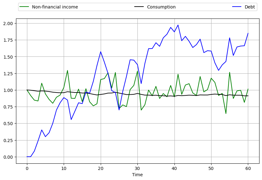
Observe that consumption is considerably smoother than income.

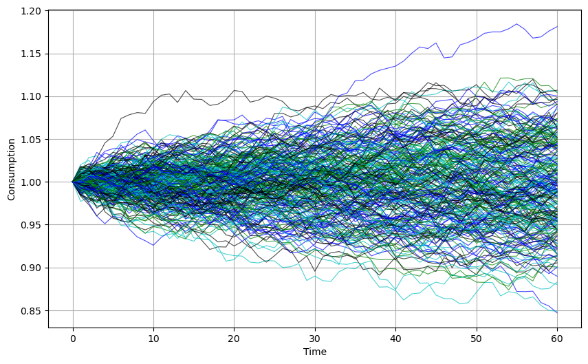
The figure below shows the consumption paths of 250 consumers with independent income streams

fig, ax = plt.subplots(figsize=(10, 6))

b_sum = np.zeros(T+1)
for i in range(250):
    w, b, c = time_path(T)  # Generate new time path
    rcolor = random.choice(('c', 'g', 'b', 'k'))
    ax.plot(c, color=rcolor, lw=0.8, alpha=0.7)

ax.grid()
ax.set(xlabel='Time', ylabel='Consumption')

plt.show()

60.3.1. Hall’s Representation#

Hall [Hall, 1978] suggested an insightful way to summarize the implications of LQ permanent income theory.

First, to represent the solution for $b_t$, shift (60.9) forward one period and eliminate $b_{t+1}$ by using (60.2) to obtain

If we add and subtract ${\beta }^{-1}(1-\beta )\sum _{j=0}^{\mathrm{\infty }}{\beta }^j{\mathbb{E}}_t{y}_{t+j}$ from the right side of the preceding equation and rearrange, we obtain

The right side is the time $t+1$ innovation to the expected present value of the endowment process $\{y_t\}$.

We can represent the optimal decision rule for $(c_t,b_{t+1})$ in the form of (60.16) and (60.8), which we repeat:

Equation (60.17) asserts that the consumer’s debt due at $t$ equals the expected present value of its endowment minus the expected present value of its consumption stream.

A high debt thus indicates a large expected present value of surpluses $y_t-c_t$.

Recalling again our discussion on forecasting geometric sums, we have

Using these formulas together with (60.3) and substituting into (60.16) and (60.17) gives the following representation for the consumer’s optimum decision rule:

Representation (60.18) makes clear that

• The state can be taken as $(c_t,z_t)$.

  • The endogenous part is $c_t$ and the exogenous part is $z_t$.

  • Debt $b_t$ has disappeared as a component of the state because it is encoded in $c_t$.

• Consumption is a random walk with innovation $(1-\beta )U(I-\beta A{)}^{-1}C{w}_{t+1}$.

  • This is a more explicit representation of the martingale result in (60.6).

60.3.2. Cointegration#

Representation (60.18) reveals that the joint process $\{c_t,b_t\}$ possesses the property that Engle and Granger [Engle and Granger, 1987] called cointegration.

Cointegration is a tool that allows us to apply powerful results from the theory of stationary stochastic processes to (certain transformations of) nonstationary models.

To apply cointegration in the present context, suppose that $z_t$ is asymptotically stationary 3.

Despite this, both $c_t$ and $b_t$ will be non-stationary because they have unit roots (see (60.11) for $b_t$).

Nevertheless, there is a linear combination of $c_t,b_t$ that is asymptotically stationary.

In particular, from the second equality in (60.18) we have

Hence the linear combination $(1-\beta )b_t+c_t$ is asymptotically stationary.

Accordingly, Granger and Engle would call $\left[\begin{array}{cc}(1-\beta )& 1\end{array}\right]$ a cointegrating vector for the state.

When applied to the nonstationary vector process ${\left[\begin{array}{cc}{b}_t& c_t\end{array}\right]}^{\prime }$, it yields a process that is asymptotically stationary.

Equation (60.19) can be rearranged to take the form

Equation (60.20) asserts that the cointegrating residual on the left side equals the conditional expectation of the geometric sum of future incomes on the right 4.

60.3.3. Cross-Sectional Implications#

Consider again (60.18), this time in light of our discussion of distribution dynamics in the lecture on linear systems.

The dynamics of $c_t$ are given by

or

The unit root affecting $c_t$ causes the time $t$ variance of $c_t$ to grow linearly with $t$.

In particular, since $\{{\hat{w}}_t\}$ is IID, we have

where

When $\hat{\sigma }>0$, $\{c_t\}$ has no asymptotic distribution.

Let’s consider what this means for a cross-section of ex-ante identical consumers born at time $0$.

Let the distribution of $c_0$ represent the cross-section of initial consumption values.

Equation (60.22) tells us that the variance of $c_t$ increases over time at a rate proportional to $t$.

A number of different studies have investigated this prediction and found some support for it (see, e.g., [Deaton and Paxson, 1994], [Storesletten et al., 2004]).

60.3.4. Impulse Response Functions#

Impulse response functions measure responses to various impulses (i.e., temporary shocks).

The impulse response function of $\{c_t\}$ to the innovation $\{w_t\}$ is a box.

In particular, the response of $c_{t+j}$ to a unit increase in the innovation $w_{t+1}$ is $(1-\beta )U(I-\beta A{)}^{-1}C$ for all $j\ge 1$.

60.3.5. Moving Average Representation#

It’s useful to express the innovation to the expected present value of the endowment process in terms of a moving average representation for income $y_t$.

The endowment process defined by (60.3) has the moving average representation

where

• $d(L)=\sum _{j=0}^{\mathrm{\infty }}{d}_j{L}^j$ for some sequence $d_j$, where $L$ is the lag operator 5

• at time $t$, the consumer has an information set 6 $w^t=[w_t,w_{t-1},\dots ]$

Notice that

It follows that

Using (60.24) in (60.16) gives

The object $d(\beta )$ is the present value of the moving average coefficients in the representation for the endowment process $y_t$.

60.4.1. Example 1#

Assume as before that the consumer observes the state $z_t$ at time $t$.

In view of (60.18) we have

Formula (60.26) shows how an increment ${\sigma }_1{w}_{1t+1}$ to the permanent component of income $z_{1t+1}$ leads to

• a permanent one-for-one increase in consumption and

• no increase in savings $-b_{t+1}$

But the purely transitory component of income ${\sigma }_2{w}_{2t+1}$ leads to a permanent increment in consumption by a fraction $1-\beta$ of transitory income.

The remaining fraction $\beta$ is saved, leading to a permanent increment in $-b_{t+1}$.

Application of the formula for debt in (60.11) to this example shows that

This confirms that none of ${\sigma }_1{w}_{1t}$ is saved, while all of ${\sigma }_2{w}_{2t}$ is saved.

The next figure displays impulse-response functions that illustrates these very different reactions to transitory and permanent income shocks.

r = 0.05
β = 1 / (1 + r)
S = 5   # Impulse date
σ1 = σ2 = 0.15

@jit
def time_path(T, permanent=False):
    "Time path of consumption and debt given shock sequence"
    w1 = np.zeros(T+1)
    w2 = np.zeros(T+1)
    b = np.zeros(T+1)
    c = np.zeros(T+1)
    if permanent:
        w1[S+1] = 1.0
    else:
        w2[S+1] = 1.0
    for t in range(1, T):
        b[t+1] = b[t] - σ2 * w2[t]
        c[t+1] = c[t] + σ1 * w1[t+1] + (1 - β) * σ2 * w2[t+1]
    return b, c


fig, axes = plt.subplots(2, 1, figsize=(10, 8))
titles = ['permanent', 'transitory']

L = 0.175

for ax, truefalse, title in zip(axes, (True, False), titles):
    b, c = time_path(T=20, permanent=truefalse)
    ax.set_title(f'Impulse reponse: {title} income shock')
    ax.plot(c, 'g-', label="consumption")
    ax.plot(b, 'b-', label="debt")
    ax.plot((S, S), (-L, L), 'k-', lw=0.5)
    ax.grid(alpha=0.5)
    ax.set(xlabel=r'Time', ylim=(-L, L))

axes[0].legend(loc='lower right')

plt.tight_layout()
plt.show()

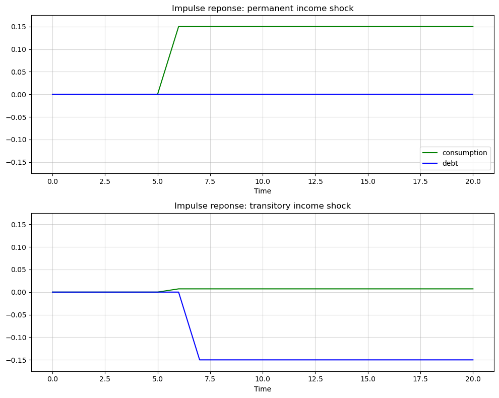
Notice how the permanent income shock provokes no change in assets $-b_{t+1}$ and an immediate permanent change in consumption equal to the permanent increment in non-financial income.

In contrast, notice how most of a transitory income shock is saved and only a small amount is saved.

The box-like impulse responses of consumption to both types of shock reflect the random walk property of the optimal consumption decision.

60.4.2. Example 2#

Assume now that at time $t$ the consumer observes $y_t$, and its history up to $t$, but not $z_t$.

Under this assumption, it is appropriate to use an innovation representation to form $A,C,U$ in (60.18).

The discussion in sections 2.9.1 and 2.11.3 of [Ljungqvist and Sargent, 2018] shows that the pertinent state space representation for $y_t$ is

where

• $K:=$ the stationary Kalman gain

• $a_t:=y_t-E[y_t|y_{t-1},\dots ,y_0]$

In the same discussion in [Ljungqvist and Sargent, 2018] it is shown that $K\in [0,1]$ and that $K$ increases as ${\sigma }_1/{\sigma }_2$ does.

In other words, $K$ increases as the ratio of the standard deviation of the permanent shock to that of the transitory shock increases.

Please see first look at the Kalman filter.

Applying formulas (60.18) implies

where the endowment process can now be represented in terms of the univariate innovation to $y_t$ as

Equation (60.29) indicates that the consumer regards

• fraction $K$ of an innovation $a_{t+1}$ to $y_{t+1}$ as permanent

• fraction $1-K$ as purely transitory

The consumer permanently increases his consumption by the full amount of his estimate of the permanent part of $a_{t+1}$, but by only $(1-\beta )$ times his estimate of the purely transitory part of $a_{t+1}$.

Therefore, in total, he permanently increments his consumption by a fraction $K+(1-\beta )(1-K)=1-\beta (1-K)$ of $a_{t+1}$.

He saves the remaining fraction $\beta (1-K)$.

According to equation (60.29), the first difference of income is a first-order moving average.

Equation (60.28) asserts that the first difference of consumption is IID.

Application of formula to this example shows that

This indicates how the fraction $K$ of the innovation to $y_t$ that is regarded as permanent influences the fraction of the innovation that is saved.